Possible Insight

General Circulation Models (GCMs) play a key role in climate change policy. Their results shape expectations of future warming from CO2 emissions and thus the justification of which policy alternatives are worthwhile. Obviously, understanding their accuracy is important for selecting the optimal policies.

Unsurprisingly, there is a substantial and contentious literature on this topic. Here are two “pro” references: (1) (2). Here are two “con” references (1) (2). I’m not going to debate pro and con here [UPDATE 9/11/2019: I catalog the con literature here]. Rather, I’m going to measure model accuracy in a different way. I have not seen anyone simply treat GCMs as black box time series prediction algorithms, then apply prediction contest ranking procedures to them. (I apologize if I missed such a treatment.)

In general, we have a lot of experience ranking statistical and machine learning prediction models. Kaggle (homepage, Wikipedia), acquired by Google in 2017, has run 100s of prediction contests since 2010–many with significant commercial prizes. Software companies like DataRobot use an automated Kaggle-like mechanic to evaluate 100s of alternative prediction models for business problems at enterprise and government customers. So in cases where predictions drive important decisions, this approach is pretty widely accepted.

All I’m going to do is apply it to GCMs. I treat each of 42 model runs in one of the official CMIP5 project archives as the output of a prediction algorithm. Then I run a Kaggle-like contest to see how these runs compare to predictions from two simple algorithms that any high schooler familiar with Excel could run: an arithmetic average and linear trend.

I “grade” using the following rubric:

• A: beats trend on both absolute and squared error.
• B: beats trend on either absolute or squared error but worse on the other.
• C: beats the average but worse than trend on both absolute and squared error.
• D: worse than the average on either absolute or squared error.
• F: worse than the average on both absolute and squared error.

(Note, this grade only applies to how well a model predicts average temperatures. There are undoubtedly other important dimensions to model quality. But to the extent that these temperature predictions provide justification for various policy responses, these grades have some validity.)

 

Results

In the spirit of “bottom line up front”, I’ll start with the results and then describe the methodology that produced them. But please note, I actually wrote up the methodology first–before even running the analysis–so that, to the greatest extent possible, I didn’t unconsciously bias the results.

At a high level, we have a good news/bad news situation for the GCMs:

• Good News: Only 2 of the model runs received an F (Series 28 and 17) and only 1 received a D (Series 5). So 93% of the runs can beat a simple historical average.
• Bad News: Not a single model run could beat a linear trend on either absolute or squared error. So 93% of the runs received a C.
• More Bad News. The GCMs are systemically too high in their forecast. The average cumulative (but not absolute) error of these models was 0.115 deg C too high. For comparison, the linear model was only .00298 deg C too high. 70% of 42 GCMs had average cumulative errors greater than 0.100 deg C too high. Only 4 had cumulative predictions that were too low over the test period.

Why would the linear model beat the much more sophisticated GCMs? Well first, the linear model is actually rather good. The mean absolute error is only 0.100 deg C. The standard deviation is .091. The maximum is 0.441. So just by knowing the historical data, one can predict the average monthly temperature 15 years out within 0.100 deg on average, 97.5% of the predictions are within 0.282 deg, and no prediction is off by more than 0.441 deg.

As detailed in the Methods section, the linear model calculates the trend for each month over the 30 years up through June 2004 and then extrapolates it to predict temperatures over the next 15 years. Below is a grid showing the monthly trends from the training and test periods, as well as their differences.

	Jan	Feb	Mar	Apr	May	Jun	July	Aug	Sep	Oct	Nov	Dec
Training	.016	.021	.018	.017	.015	.017	.018	.019	.016	.019	.016	.015
Test	.021	.026	.029	.023	.023	.014	.019	.023	.015	.017	.010	.023
Difference	.005	.005	.010	.006	.009	-.003	.001	.004	-.001	-.002	-.006	.008

 

The trends just don’t differ much from training to test period. The average absolute difference in trend is .005. Unsurprisingly, a linear model calculated from the training period does pretty well in the test period.

You can appreciate the consistency in these plots of the January and July temperatures over both periods, with the trend from the training period only superimposed.

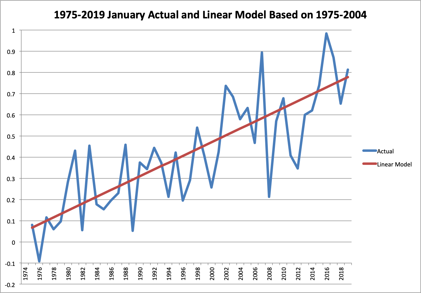
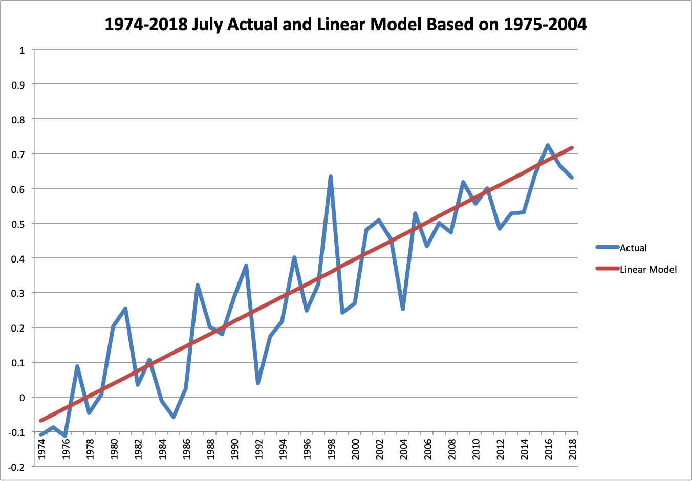
Visually, it’s hard to even distinguish that the trend line is not actually calculated across the entire period.

To see how the GCMs stack up, here is the “leaderboard” from the absolute error comparison. I’ve put it in terms of mean absolute error for ease of interpretation–it’s the average number of deg C that the predictions for that model differs from actual.

Model	Mean Absolute Error
Trend	0.100
Series 15	0.116
Series 14	0.135
Series 27	0.136
Series 25	0.139
Series 41	0.144
Series 34	0.146
Series 19	0.153
Series 24	0.158
Series 10	0.161
Series 11	0.162
Series 13	0.162
Series 18	0.166
Series 16	0.168
Series 20	0.168
Series 23	0.169
Series 21	0.172
Series 31	0.174
Series 42	0.175
Series 40	0.176
Series 29	0.181
Series 39	0.185
Series 36	0.187
Series 22	0.191
Series 9	0.194
Series 35	0.198
Series 3	0.204
Series 26	0.211
Series 12	0.213
Series 38	0.215
Series 37	0.216
Series 8	0.241
Series 7	0.244
Series 32	0.249
Series 1	0.261
Series 2	0.264
Series 30	0.266
Series 33	0.292
Series 4	0.295
Series 6	0.327
Series 5	0.370
Average	0.380
Series 28	0.401
Series 17	0.422

 

6 models are within 1.5X the mean error of the trend. I suppose I could give these models a C+ grade. Though 18 models have more than 2X the mean error of the trend, which I would call a C-.

It’s a little surprising that no model beat the trend and I was concerned that I might have made a serious error in processing data from the GCM runs for the predictions. So I constructed a double check. The median performing models on absolute error are Series 39 and 36 (the 21st and 22nd best). Coincidentally, the median performing models on squared error are Series 36 and 39. I calculated the linear trends of these two models during the training and test periods from the original source data, before any processing, and compared them to the trends from the actual temperature data.

	Jan	Feb	Mar	Apr	May	Jun	July	Aug	Sep	Oct	Nov	Dec
Training	.016	.021	.018	.017	.015	.017	.018	.019	.016	.019	.016	.015
Series 36	.016	.018	.016	.016	.016	.019	.019	.019	.020	.020	.018	.020
Series 39	.026	.025	.024	.024	.021	.023	.022	.021	.024	.023	.026	.026
Test	.021	.026	.029	.023	.023	.014	.019	.023	.015	.017	.010	.023
Series 36	.038	.043	.045	.045	.035	.039	.047	.037	.045	.036	.036	.031
Series 39	.010	.022	.030	.016	.016	.022	.023	.024	.023	.023	.016	.016
Difference	.005	.005	.010	.006	.009	-.003	.001	.004	-.001	-.002	-.006	.008
Series 36	-.017	-.017	-.016	-.022	-.011	-.025	-.028	-.014	-.030	-.018	-.027	-.007
Series 39	.011	.004	-.001	.007	.007	-.008	-.004	-.001	-.008	-.006	-.006	.007

 

During the test period, the average difference in trend from actual for Series 36 is .017 and for Series 39 is .011.  So the median GCM model runs have trends during the test period that are off by 2-3X as much as the extrapolated trend from the training period. Therefore, it’s not too surprising that the GCMs as a whole scored poorly against the trend.

Graphically, we can compare actual and the extrapolated trend to those of the best GCM model and one of the median GCM models. Series 15 had an absolute error only 16% more than the extrapolated trend. Series 36 was 88% more. These differences are pretty clear on graphs for January and July of the test period.

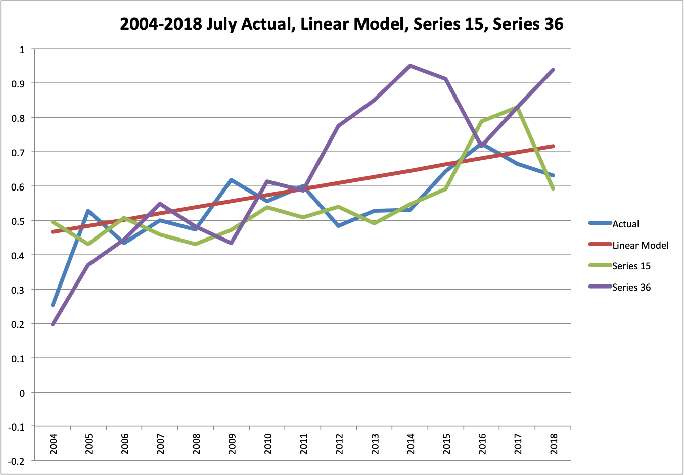
You can see that Series 15 does a pretty decent job of following actuals with a few mistakes, while Series 36 seems to go the opposite of actual in many ways. The exratrapolated trend does a decent job across the board. These checks makes me more confident that I didn’t make a large computation error.

In addition to testing individual models, I also tested ensembles. As I understand it, climate modelers construct some runs to represent different scenarios that only have a modest chance of occurring and the collection of models as a whole are designed to capture the possible variation. First, I tested the entire ensemble of 42 models. In terms of absolute error, this model would have ranked 13th, with 64% more error than the linear model. In terms of squared error, it would have ranked 9th with 2.1X as much squared error.

I also constructed a “Top 10” ensemble of Series 10, 11, 14, 15, 19, 24, 25, 27, 34, and 41. I cheated a little bit and used the ranking from the test period. Ideally, I would have selected the top 10 from the training period, but that would have been substantially more work because I hadn’t already computed errors from the training period for all the GCMs. In any case, this cheat overestimates how good the ensemble is. With this cheat, it ranked 2nd in absolute error, still 14% behind the linear model, and 3rd in squared error, still 19% behind the linear model.

These results argue that the GCMs, at least the ones used to produce the CMIP5 archive from 2013, do not have predictive skill relative to a linear trend, at least over a 15 year time horizon. Also, they systematically predict temperatures that are too high. I provide some final thoughts after the Methods section.

 

Methods

Training and Test periods

In statistical and machine learning, one typically uses a “training” period and a “test” period to evaluate models. 15 years of monthly predictions for the “test” period seems like a reasonable number and we obviously want to use the latest data. That implies a test period from July 2004 to June 2019.

As far as I can tell, all the data in the CMIP5 archive is as of March 15, 2013 (reference, pg 4). So testing 2004 to 2019 would seem to violate a strict training-test separation. However, GCMs aren’t “trained” in the same way as learning algorithms. They are supposed to be bottom up models of physical processes. Also, most of the models appear to have been developed over a long period. So while the model builders had some information from 2004 to 2013, it probably wasn’t directly incorporated into the models as it would have been for learning algorithms. In any case, this choice can only possibly bias my analysis towards overestimating GCM prediction accuracy.

Moreover, I use a calibration step vaguely analogous to “training” in my analysis. I calculate the average recorded historical temperature for each calendar month in the 30-year period up though June 2004. Then I calculate the same averages for each GCM run. I subtract them to compute a monthly offset that “centers” each model’s monthly predictions on the 30-year training period. To evaluate accuracy, I compare the model’s monthly prediction plus the monthly offset to the actual temperature anomaly during the test period. (Note: this also takes care of the fact that the model output is temperature and the actual measurements are in terms of temperature anomalies).

Temperature Data Set

In addition to choosing the training-test split and applying the centering procedure, there are two more key decisions in my analysis. The first is choosing a source for the “actual” temperature data. There are three well-known thermometer-based surface temperature data sets: GISS, CRU, and Berkeley Earth. Initially, I was planning to average their respective global land and ocean datasets. Then I started thinking. These products pull mostly from the same raw thermometer data and then apply different procedures for calculating a single global temperature. So averaging them is mostly averaging their procedures, rather than their underlying data. It wasn’t clear to me that averaging procedures would produce a better result.

I went to the literature for insight and found this article from the Lead Scientist at Berkeley Earth. In it, he shows that the Berkeley procedure produces less error when applied to temperature simulations from GCMs, where you already know the temperature field. Given that we’re comparing GCM data to actuals, that seems pretty compelling. So I use Berkeley Earth by itself. I pulled the data from this file on 8/11/2019. The conversion to Excel is here. I then broke it into a training version from July 1974 to June  2004 and a test version from July 2004 to June 2019. The training version also computes the monthly mean and monthly least squares trend anomalies.

CO2 Emissions Scenario

The second key decision is CO2 emissions scenario. Obviously, GCMs need to know how much CO2 humans will emit to calculate the temperature. We don’t know exactly what they will be in the future, so we have to choose a forecast. The IPCC uses “Representative Concentration Pathways” (RCPs) for this purpose. This paper reviews the scenarios.

The Mauna Loa data show CO2 increasing from 352 to 409 ppm from 1988 to 2018. That’s 1.90 ppm per year. At that rate, the concentration would reach 565 ppm in 2100, almost exactly double the pre-industrial value of 280 ppm. RCP 4.5 has CO2 concentrations stabilizing at 550 ppm in 2100, which is by far the closest RCP. So I use RCP 4.5.

The official CMIP5 model archives are here. However, they use a data format that I am not familiar with and Willis Eschenbach has already downloaded the data and converted the RCP 4.5 results to Excel here. I downloaded his file on 8/11/2019 and archived it here. I also broke it into training and test versions. The training version computes the average monthly temperatures for each model and subtracts it from the actual monthly average anomaly to compute the offset for the centering step.

Analysis

The test file performs the analysis. The first tab has the original data from each GCM run during the test period. The second tab adds in the average and trend model predictions. The third contains the monthly offsets for each GCM run and the fourth applies the offsets. The fifth and sixth calculate the absolute and squared errors. The seventh and eighth show the leaderboard for the absolute and squared measurements with the average and trend models highlighted in yellow and green.

 

Final Thoughts

• Assuming I have not made any serious conceptual or computational errors, it does not appear that the generation of GCMs from the early 2010s does a very good job of predicting temperatures on a 15-year time horizon.
• Moreover, these models systematically predict temperatures that are too high.
• I am modestly confident that I have not made any serious conceptual errors.
• I am pretty sure that I have made computational errors somewhere. I am only somewhat confident that these are not serious enough to affect the main conclusion.
• Regardless of my conceptual or computational errors in this specific analysis, I think this methodology is worth pursuing. If our policy choices now depend on our beliefs about the amount of future warming caused by human CO2 emissions, we should apply our best knowledge of how to build predictive models to climate modeling.
• I strongly suspect that if top scientists from statistical and machine learning collaborated with  top scientists from climate modeling, we would see a substantial improvement in the ability of GCMs to make skillful predictions.